Case study
Demand Forecasting System
Supply-chain demand forecasts with LightGBM and XGBoost, plus a published naive-baseline benchmark.
At a glance
Plain summary for recruiters and visitors. Technical detail follows below.
- What it is
- I built a supply chain demand forecasting pipeline with tree models and simple baselines. On a fixed benchmark series it slightly beats a naive mean forecast.
- What I owned
- Solo end to end. Lag features, LightGBM and XGBoost training, baseline benchmarks, optional agentic model pick, and the portfolio forecast demo.
- Why it matters
- Even a small edge over naive mean can reduce waste when the same logic runs across many SKUs. The case study reports honest one-step numbers before any multi-step serving claim.
- Try it on this page vs full project
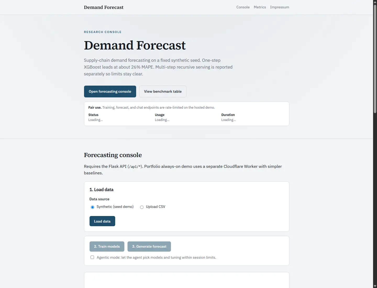
- The chart demo uses lightweight JavaScript models on curated series. The published about 26% MAPE table comes from the full XGBoost and LightGBM stack on request.
Problem
Supply chain teams waste time on manual forecasts that miss demand swings and inflate inventory cost.
Method
Combined lag features with LightGBM and XGBoost, plus classical baselines and an agentic mode for model selection. Benchmarked one-step skill against naive mean and seasonal naive on a fixed seed.
Result
About 26% MAPE one-step (XGBoost) on the published synthetic protocol, slightly ahead of naive mean. Multi-step recursive serving is reported separately so limits stay clear.
Architecture
How the system is shaped. Full implementation stays private.
Step 1
Ingest
Time series demand feeds with validation and scale checks.
Step 2
Features
Lags, calendar effects, and rolling stats for tree models.
Step 3
Models
LightGBM, XGBoost, classical baselines, optional agentic model pick.
Step 4
Evaluate
MAPE/WAPE versus naive mean and seasonal naive on a fixed seed before serving.
One-step MAPE vs baselines
Fixed synthetic seed 42, 730 days, 80/20 split, first 30 test days, teacher-forced lags. Multi-step recursive forecasts are weaker for trees on this series. The published table is one-step MAPE only.
| Model | MAPE | Note |
|---|---|---|
| XGBoost | 26.2% | Best in this run |
| Naive mean | 26.9% | |
| LightGBM | 30.7% | |
| Seasonal naive (p=7) | 119.1% |
Algorithm
Gradient-boosted demand regression
Tabular time-series features into LightGBM/XGBoost with optional ensemble blending and agentic model choice.
X, y = build_lag_features(series)
model = LightGBM.fit(X_train, y_train)
yhat = model.predict(X_test)
mape = mean(abs(y_test - yhat) / y_test)
compare(mape, naive_mean_mape, seasonal_naive_mape)
Key logic
Compact illustrative snippet (Lag and calendar features (illustrative)). Not the full codebase.
def build_lag_features(series, lags=(1, 7, 14), rolls=(7, 28)):
    df = pd.DataFrame({"y": series})
    for k in lags:
        df[f"lag_{k}"] = df["y"].shift(k)
    for w in rolls:
        df[f"roll_mean_{w}"] = df["y"].rolling(w).mean()
    df["dow"] = df.index.dayofweek
    df["month"] = df.index.month
    return df.dropna()
Stack
Try a live forecast
Free Cloudflare demo on a curated series. Pure JS seasonal, Holt, and lag-ridge only. The published case-study table is one-step XGBoost at about 26% MAPE on a different synthetic protocol.
Scenario
Model
Source code
Full source is available to hiring managers on request. The public page shows architecture, algorithms, and compact proofs only.